Section 1: Methodology
The Institute on Taxation and Economic Policy (ITEP) has engaged in research on tax issues since 1980, with a focus on the distributional consequences of current law and proposed changes. Much of ITEP’s research, including this report, is based on ITEP’s proprietary microsimulation tax model, which estimates the amount of federal, state, and local taxes paid by residents of every state at different income levels under current law and alternative tax proposals. The ITEP Tax Microsimulation Model’s structure mirrors models at the federal level maintained by the congressional Joint Committee on Taxation, the U.S. Treasury Department, and the Congressional Budget Office, and at the state level by the Minnesota Department of Revenue and other state agencies. This section describes the ITEP Tax Microsimulation Model and the techniques used in modeling the tax systems of the 50 states and the District of Columbia.
About Who Pays?
Since 1996, ITEP has published a series of reports that measure and compare the distribution, or incidence, by income level, of state and local taxes in all 50 states and the District of Columbia. The reports, entitled Who Pays?, each show a single-year snapshot of state and local tax incidence.
This report examines 2024 tax law as of January 1, 2024. Those tax parameters are applied to the population and economy of each state at 2023 levels, with inflation-indexed parameters modeled at 2023 levels for the sake of consistency. In other words, the report shows the amount of income, consumption, and property taxes that would have been paid by residents in 2023 with the January 1, 2024 law in place. This decision to use 2023 economic data was made to avoid having to rely on economic and revenue forecasts for 2024 that are unavoidably speculative. An accurate summary of the report’s approach is “2024 tax law at 2023 income levels.”
This is the 7th edition of this report.
What’s New?
Over the seven editions of Who Pays?, states’ tax systems have been amended, their economies have changed, and ITEP’s methodologies have evolved. Readers seeking to understand why their state’s results may look different from previous editions of the report, and the extent to which results from past editions are comparable to the results in this one, should be aware of the following five factors:
- State and local tax laws have changed significantly since the 6th edition of this report was published. The previous edition of Who Pays? included laws enacted through September 10, 2018. This report includes laws enacted through January 1, 2024, provided they will be in effect for 2024.
- Economic and social changes have affected the results. They have changed the underlying distribution of income that is used as the measuring stick for tax incidence. They have also expanded, contracted, or otherwise altered various tax bases. Cigarette taxes, for example, have declined as a share of income since the previous edition because of falling smoking rates and substantial wage growth. The previous edition of Who Pays? used economic and demographic data from 2015. This edition uses 2023 data.
- A range of minor taxes that were excluded from previous editions are now included in the scope of this study. Taxes on insurance premiums, natural resource extraction, and real estate transfers are the most notable additions, though a multitude of smaller taxes on everything from parking to snowmobile sales are now reflected as well. The previous edition included approximately 90 percent of all state and local tax revenues. The comparable figure for this edition is 99.7 percent.
- While the methodology used in this study is very similar to the approach used in previous editions of the report, this edition reflects the availability of new data sources, new methods for integrating data, and some modifications in modeling approach based on advancements in methodological research. For instance, we have improved our method for measuring in-state business activity and, by extension, business-paid taxes associated with nonresident firm owners. We have also built a new estate tax module that better measures the relationship between taxable estate value and income. We have added additional nuance to our corporate tax modeling that more fully considers apportionment rules. We have also improved our measurement of residential rental property taxes. These changes improve our measurement of tax incidence but, in the context of the analysis of entire tax systems presented here, their impact is small.
- Unlike some earlier editions of Who Pays?, this study does not include a “federal deduction offset” reflecting the federal deduction for state and local taxes (SALT). This effect was removed from the 6th edition of Who Pays?, published in 2018, because the $10,000 SALT deduction cap imposed by the federal Tax Cuts and Jobs Act of 2017 prevented the deduction from serving as a generalized offset of state and local taxes and significantly reduced its effect on tax incidence. We have also left the offset effect out of this edition of the study, though its significance has increased since 2018 as pass-through business owners have increasingly regained indirect access to the deduction through various workarounds. Inclusion of the offset would reveal state and local tax systems to be more regressive than the data in this study indicate.
Taxes Included in the Study
This is a study of state and local taxes. We view states and their localities together as an integrated whole because state and local finances are highly intermingled, and localities derive their taxing authority from the state. States vary considerably in the rules they set for local revenue raising, and some states choose to leave more revenue-raising responsibility to local governments than others.
Both states and localities rely on a broad range of tax and non-tax revenue sources. Because of this, any tax incidence analysis requires a definition of what will be considered a tax within the scope of the study. For this purpose, we employ a definition of taxes that is nearly identical to the one used by the U.S. Census Bureau in its Survey of State and Local Government Finances. There is 99.2 percent overlap in the definition of taxes used by the Census and the one we employ in this study.
This study therefore includes all the major taxes levied by state and local governments, such as personal income taxes, corporate taxes, sales taxes, and property taxes—as well as comparatively minor levies such as insurance premiums taxes, transfer taxes, and estate and inheritance taxes. We depart slightly from the Census definition in excluding hunting, fishing, and other non-business licenses. On the other hand, we add two additional revenue sources to our definition that help us achieve greater consistency in our cross-state comparisons: payments in lieu of taxes made by the Tennessee Valley Authority, and the implicit tax charged via mark-up at state-owned liquor stores. The latter is calculated using a combination of data and analysis from the Distilled Spirits Council and state liquor control agencies.
After defining the scope of levies to be included in the study, we collect and sort data on the revenue yield of those levies. The Census government finance data are generally not reported at a fine enough level of detail for purposes of tax modeling, and thus our primary source of this information comes from a wide range of reports published by state and local revenue departments, fiscal offices, budget offices, and assessors’ offices, and sometimes from other agencies with narrow tax collection authority, such as departments of transportation.
With these baseline data in place, we then turn to the Census data to both supplement and verify the information collected from the primary sources just named. Part of this process involves reconciling the data we have collected with the data reported by Census. This is helpful in avoiding both the omission, and double counting, of tax dollars. The result is a comprehensive database of state and local revenue collections, across all states, that is unrivaled in its scope, detail, and accuracy.
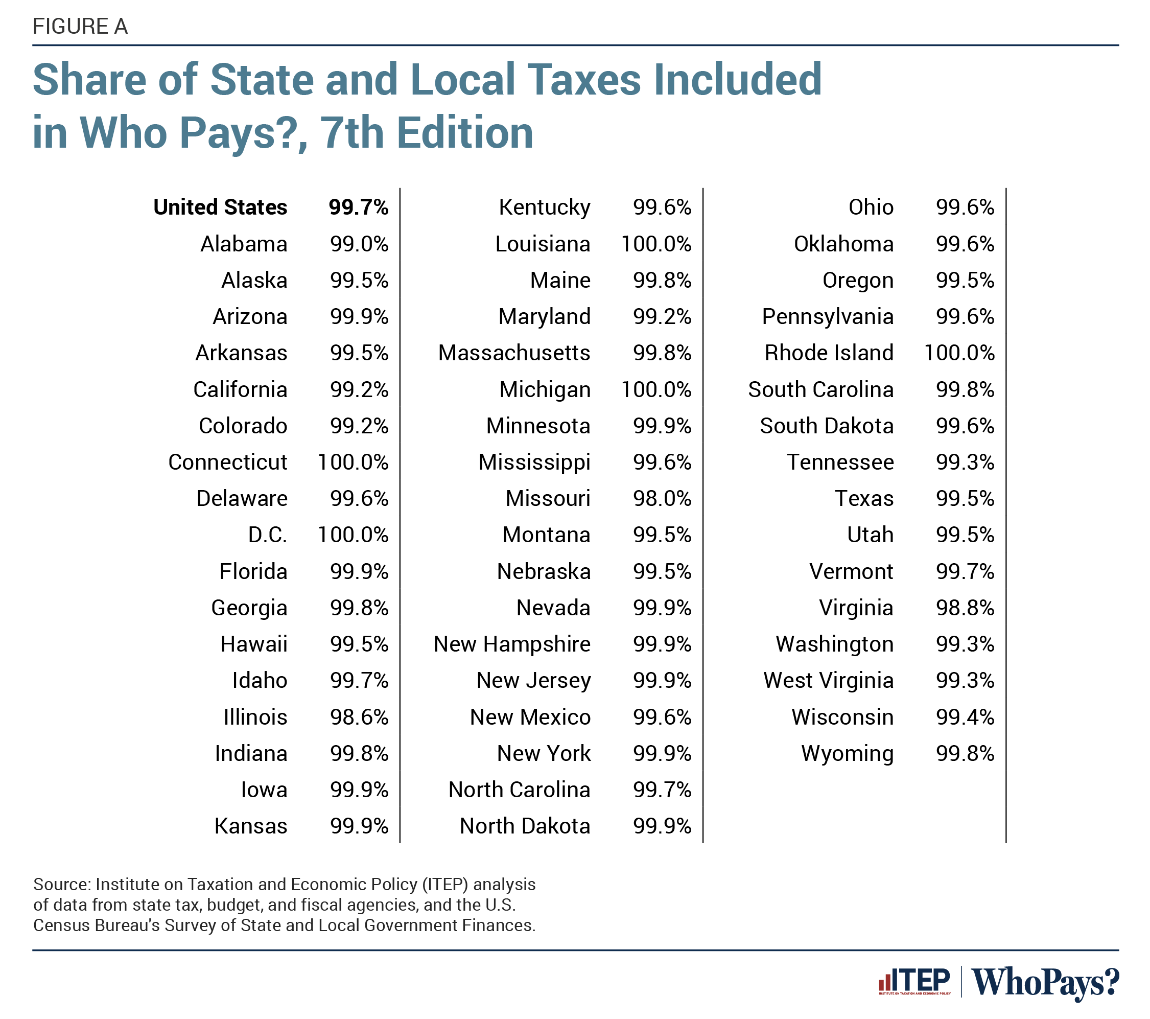
In checking our data against Census, we occasionally find small amounts of revenue reported by Census that we were unable to identify in any state or local revenue or budget report. Most often, these are dollars reported under the broad categories of “other selective sales” or “taxes not elsewhere classified”—categories too broad to be used in detailed tax modeling. These unidentified tax dollars add up to just 0.3 percent of all state and local tax dollars nationwide. In other words, our study includes 99.7 percent of all tax collections (using the ITEP definition of taxes described above). Because the 0.3 percent of unidentified taxes are likely to be consumption taxes of various types, we expect that their inclusion in the study would worsen our findings of regressivity—though only to a trivial extent given the small amount of revenue involved.
Figure A shows the share of total state and local tax revenue included in our analysis of tax incidence, for the United States and broken down by state and the District of Columbia (DC). Our study captures between 98 and 100 percent of the tax revenues raised in each of the 50 states and DC, with 99.7 percent of all state and local tax revenue included nationwide.
For purposes of reporting data in this study, the wide range of taxes analyzed are grouped into four broad categories: sales and excise taxes, property taxes, income taxes, and other taxes. Most of these categories are further subdivided in our detailed tables to provide readers with additional information about what is driving the overall results. The following list is meant to help readers broadly understand what is presented on each line of the detailed tables.
Sales and Excise Taxes
General Sales—Individuals: General sales taxes on final consumer purchases, net of sales tax credits and rebates
Other Sales & Excise—Ind.: Consumption taxes with narrower bases affecting final consumer purchases, including but not limited to taxes on insurance premiums; utilities; restaurant meals; short-term lodging; vehicle rentals; vehicle purchases; cigarettes; other tobacco; vape products; alcohol (including the implicit tax revenue generated by state liquor stores); cannabis; soda; gambling (excluding lotteries); motor fuel; tires; taxi and rideshare rides; hazardous materials
Sales & Excise on Business: Broad gross receipts taxes; the portion of general and selective consumption taxes paid by businesses on their inputs
Property Taxes
Home, Rent, Car—Individuals: Real estate property taxes and transfer taxes on owner-occupied homes and vacation homes, net of property tax rebates; the portion of residential real estate taxes passed through to tenants, net of property tax rebates; motor vehicle taxes and registration charges paid on individual, non-commercial vehicles
Other Property Taxes: Property taxes paid by businesses on real estate, vehicles, and certain other tangible property; the portion of residential real estate taxes falling on landlords; real estate transfer taxes paid on business and residential rental property; estate and inheritance taxes
Income Taxes
Personal Income Tax: Individual income taxes on both broad and narrow definitions of net income, net of income tax credits
Corporate Income Tax: Corporate income taxes and certain other business income taxes; financial institutions taxes; franchise taxes; corporate licenses
Other Taxes
Severance taxes; business and occupational licenses; alcoholic beverage licenses; amusement licenses; marriage licenses; drivers’ licenses; flat taxes assessed per person or per pay period
Definition of Family Income
Income measurement is an important part of tax incidence analysis because income is the benchmark against which effective tax rates are calculated. Federal and state tax codes’ definitions of adjusted gross income (AGI) offer relatively straightforward, ready-made definitions and are sometimes used in other organizations’ incidence analyses. But AGI is a flawed measure for this purpose because of gaps, and variation across states and over time, in what it includes. ITEP takes a more inclusive and consistent approach to measuring cash income and includes both income that is subject to tax and income that is exempt. This broader definition offers a better measurement of tax units’ ability to pay and more meaningful effective tax rate results.
Our income measurement begins with the amounts reported to IRS. But some people do not file tax returns and many more earn income that does not appear on IRS forms. For non-filers we supplement the IRS returns with observations from the American Community Survey (ACS). For components of income that are either fully or partly tax exempt, we supplement data available from the IRS with data from the ACS, Congressional Budget Office, and various administrative data sources. The generally non-taxable income items for which ITEP makes state-by-state estimates (which are included in our measure of “total income”) include: Social Security benefits, Worker’s Compensation benefits, unemployment compensation, Veterans Affairs benefits, child support, financial assistance, public assistance, and Supplemental Security Income (SSI). Our income estimates also include income that is not statutorily exempt, but that is underreported or nonreported in practice (Johns and Slemrod, 2010; Krause et al., 2022). Omission of this income would make our effective rate estimates appear artificially high.
Our reporting of income groups includes additional detail at the high end of the income distribution. The best-off 20 percent of tax units are a diverse group, including everyone from solidly middle-class couples earning $138,000 per year, all the way up to billionaires. Because of the huge variation in the incomes of the top 20 percent, tax incidence within the group varies widely.
Moreover, the best-off 20 percent of tax units enjoy roughly 60 percent of nationwide personal income while the best-off 1 percent of taxpayers alone enjoy about 20 percent of nationwide personal income. By contrast, the poorest 20 percent of tax units earn less than 3 percent of nationwide income.
The concentration of income at the top, and the variability of income levels and tax incidence within the top 20 percent, makes splitting up this group necessary for meaningful tax analysis. Small differences in the tax treatment of the best-off taxpayers can have disproportionate implications for state tax collections and incidence. In addition, many state tax codes provide special favor for the best-off 1 percent and their income composition is quite different from that of most taxpayers, as it exhibits a concentration of capital gains and business income not seen at other points in the income distribution. Considering the top fifth as a whole would gloss over these substantial differences. For these reasons, this study reports effective tax rates for three subgroups of the top 20 percent: the “Next 15 percent,” or 80th-94th percentile, the “Next 4 percent,” or 95-99th percentile, and the “Top 1 percent.”
Scope of Tax Units Included
This study groups people into tax units, which are persons or groups of people who file one tax return or, for nonfilers, who would file one tax return if they were to file. All of ITEP’s estimates are produced at the tax unit level, though we occasionally use the terms “households,” “families,” or “taxpayers” when describing our results as these terms are more familiar to most readers. Tax units can be either smaller or larger than Census’s definition of households, though on average they are smaller because the latter can include roommates or multigenerational families that file more than one tax return.
The report’s universe of taxpayers includes most, but not all, of the tax units residing in each state. It includes citizens as well as documented and undocumented immigrants, to the extent that they are included in the IRS data as ITIN filers or in the American Community Survey data that inform the nonfiler database. Dependent filers are grouped together with the tax unit that claimed them as dependents to avoid double counting and to better reflect the combined unit’s ability to pay. Tax units with negative incomes are excluded from our distributional presentation as it is not possible to calculate a meaningful effective tax rate against a negative income amount. American Indians living on federally recognized reservations are also excluded from our state distributional tables because, as sovereign nations, many tribal governments have their own systems of taxation and those tax systems are outside the scope of this study.
This study also excludes senior tax units, defined as those where the primary filer or their spouse is age 65 or older. This exclusion serves two purposes.
First, state tax structures routinely treat senior families more generously than other families. The median state asks senior citizens to pay about one-third less in personal income tax than younger families with similar incomes (Brewer et al., 2017). Property tax preferences for seniors are common as well. In some states, income and property tax preferences rise to the level of offering what amounts to a parallel tax code for senior families. Blending the very different tax rules facing seniors together with those facing younger families risks yielding an overall result that is not representative of the tax situation of either group.
Second, seniors’ economic profiles are different from those of non-seniors across a range of metrics that are important in determining effective tax rates—including homeownership, asset ownership, and spending and savings rates. For the working age population, for instance, the people most likely to spend all their earnings are lower-income families struggling to afford current expenses on low pay. For some seniors, on the other hand, all income may be spent in the current year simply because they have less need to save for the future and because they have more control than non-seniors over the amount of income they realize in a given year. The BLS Consumer Expenditure Survey data exhibit high ratios of consumption to income for senior consumer units, but those ratios can mean different things within the senior cohort than they do for non-seniors.
A similar issue is present in property tax analysis, as seniors are more likely to have paid for their homes out of past income, and to pay their property tax bills out of their accumulated wealth rather than their current incomes. A high property tax bill relative to realized annual income may not always have the same meaning for seniors that it does for non-seniors.
Had we included seniors, state tax systems would likely have been shown to be more regressive than calculated in this study. Thus, our findings of steep regressivity in consumption taxes, and meaningful regressivity in property taxes, are particularly notable and robust given the exclusion of seniors from this study’s scope.
Who Pays? Modeling Overview
The analysis contained in this study was produced using the ITEP Tax Microsimulation Model. The ITEP Model is a tool for calculating the incidence of federal, state, and local taxes across income and demographic groups. In computing its estimates, the model relies on a large database of tax returns and supplementary data that provide an accurate representation of the entire U.S. population and the populations of each state and the District of Columbia (DC).
The ITEP Model’s basic structure mirrors models at the federal level maintained by the congressional Joint Committee on Taxation, the U.S. Treasury Department, and the Congressional Budget Office, and at the state level by the Minnesota Department of Revenue and other state agencies. Microsimulation modeling is widely regarded as the best option for this kind of policy analysis because of its ability to account for overlapping and interacting tax provisions and to produce results that are representative of the full population of interest. The ITEP Model’s main distinguishing characteristic is that it can be used to produce accurate incidence and revenue estimates for income, consumption, and property taxes in every state and DC.
The following sections discuss the tax modeling performed in this study.
Personal Income Taxes
The ITEP Model’s personal income tax module contains two broad parts. The first is an extensive database of taxpayer microdata and the second is a series of tax calculators reflecting the personal income tax laws applied to those taxpayers. Applying those calculators to our database yields distributional results of the type contained in this report, and tax revenue estimates as we have reported in other studies.
The model’s starting point is a large database of taxpayer data and supplementary information. Federal tax return data from the Internal Revenue Service (IRS) were paired with observations from the U.S. Census Bureau’s American Community Survey (ACS) to create a valid representation of the U.S. population, including federal filers and nonfilers, both nationally and for every state. Weights assigned to each record in the model indicate the number of real-world tax units it represents.
These data were further supplemented through a statistical match with the ACS to gain access to data available in the ACS but not on tax returns. The entire dataset was also supplemented with imputed values based on econometric analysis of other datasets such as the Bureau of Labor Statistics’ Consumer Expenditure Survey and the Federal Reserve’s Survey of Consumer Finances.
Each record in the model includes components of personal income and a wide range of other tax items and demographic and social characteristics. The validation year of the ITEP Model’s microdata is Tax Year 2019. That is, the weights are assigned in a way that allows the model to reflect state-by-state and national targets taken from published reports for 2019 by the Internal Revenue Service, the Bureau of the Census, and other sources. At the time the model database was being constructed, the most recent years for which the IRS published the kind of detailed, state-by-state distributional data needed for model validation were 2019 and 2020. We opted for the former year as economic and social disruptions caused by COVID-19 make 2020 a very unrepresentative year. Officials at the Joint Committee on Taxation have indicated to us that they also prefer 2019 over 2020 data for this reason.
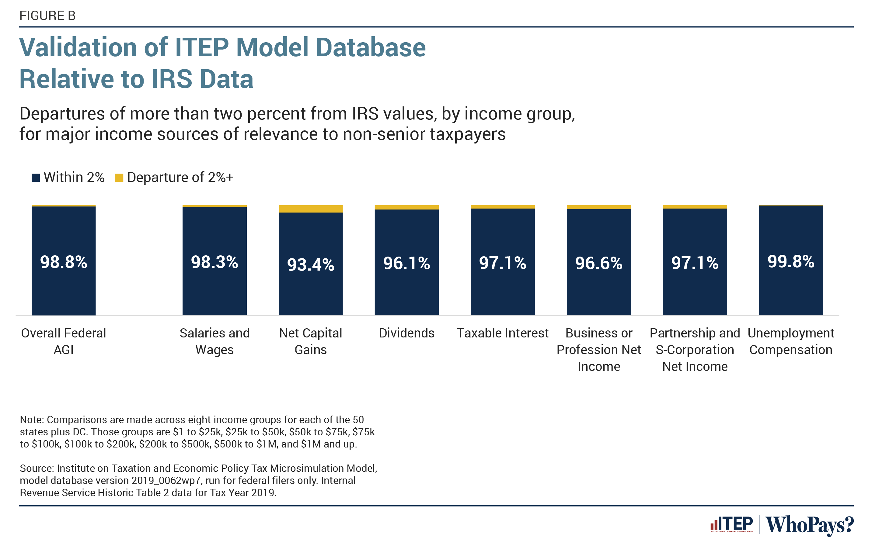
Figure B offers a demonstration of some of the results of the validation process. It shows the degree to which our model database is in alignment with data reported by the IRS for major sources of income that are of relevance to non-senior taxpayers. This figure compares the ITEP Model income values to IRS income values across 3,264 discrete points—that is, across eight measures of income, within eight different income bands, and in each of the 50 states plus DC. We are within 2 percent of IRS values in more than 97 percent of these cases. Most departures in excess of 2 percent are in the bottom part of the income scale where comparatively minor differences in income appear larger in percentage terms. This occurs most frequently in the context of capital gains and dividends, where the income amounts flowing to lower-income families are vanishingly small. Of particular note is that, for the broad measure of overall federal Adjusted Gross Income (AGI) on which most state income tax laws are based, we are within 2 percent of IRS targets in nearly 99 percent of cases.
With a valid Tax Year 2019 database in place, the next step was to age those data to Tax Year 2023 for use in this study. For years after 2019, the model adjusts the value of every component of personal income, and the weights associated with each record, to reflect targets published by the Internal Revenue Services, the Congressional Budget Office, and other sources, with variation across states to reflect differences in growth trajectories.
Our detailed tax calculators are then applied to these Tax Year 2023 data. ITEP has long maintained a series of calculators reflective of federal, state, and local personal income tax rules, the results of which are validated against available targets. These calculators were built by ITEP staff after careful review of tax forms, statutes, and recently enacted legislation in every state and DC. When these calculations are run for each unit in the personal income tax database, the result is a full picture of the distribution of taxes across the income scale in whatever jurisdiction is being analyzed.
Consumption Taxes
The ITEP Model’s consumption tax module is used to analyze the incidence of taxes levied on the purchase of goods and services and on business gross receipts. There are more than 700 tax base items available in the item database, which allow us to accurately model the wide array of different sales tax bases used at the state and local levels, as well as various smaller taxes levied on narrow categories of consumption. Most of the data in the consumption module are dollar spending values, though we also have quantity estimates for items such as motor fuel and tobacco that are often taxed based on quantity purchased rather than amount spent.
State and local consumption taxes are paid by a variety of actors, including state residents, visitors from outside the state, and businesses. Visitor estimates were derived using data from a variety of sources, with U.S. Travel Association data being the most important. Business purchase estimates were obtained using a method similar to the one laid out in Chainbridge Software (2013). The shifting of business-paid consumption taxes onto individuals is discussed later in this methodology.
While the statutory burden of excise taxes on products such as motor fuel, tobacco, and alcohol is on the seller rather than the purchaser, the final incidence of these taxes is not meaningfully different from if the tax were applied directly at the point of final sale to the individual purchaser (Chouinard et al., 2004; Kenkel, 2005; Hanson and Sullivan, 2009; Brock et al., 2016). For this reason, we treat these taxes as falling on individuals and report them on the “Other Sales & Excise—Ind.” line of the detailed tables.
For modeling consumption taxes falling directly on individuals, the primary data source informing our work is the Bureau of Labor Statistics’ Consumer Expenditure Survey (CEX). The CEX is unrivaled in the level of detail it provides (Li et al., 2010) and is thus widely used for state and local consumption tax modeling. It is the backbone of analyses conducted by agencies such as the Minnesota Department of Revenue, Maine Revenue Services, Texas Comptroller of Public Accounts, Connecticut Department of Revenue Services, Colorado Department of Revenue, and the Comptroller of Maryland.
We relied primarily on the CEX Interview Survey for imputing spending information onto the ITEP Model microdata, though we also used data from the CEX Diary Survey and various auxiliary files for purchase categories where the additional detail afforded by those sources allows for a more accurate modeling of the nuances of state and local tax law. In a handful of cases, our consumption tax modeling is informed by additional spending detail from outside the CEX. Our measurement of grocery purchases made with Supplemental Nutrition Assistance Program (SNAP) dollars, for example, is based on our analysis of the U.S. Department of Agriculture’s National Household Food Acquisition and Purchase Survey microdata.
Spending values in the model were estimated using a series of econometric equations considering household income, size, structure, homeownership status, age, race or ethnicity, geographic location, and year of survey. The imputation process proceeded in several stages, with higher-level categories estimated first and more detailed categories estimated as shares of those totals. The specification of the estimating system bears similarities to the specification of household spending demands in the EU’s indirect tax model (DeAgostini et al., 2017) while the share equations were estimated using a fractional multinomial logit algorithm developed by Bruis (2017).
One challenge of working with the CEX is that its income data tend to be of lower quality than the spending data that are the core focus of the survey (Etlidge et al., 1994). Because of this, simple comparisons of income and spending within the survey can yield invalid results. Our estimation technique included several safeguards against this outcome. Extremely low-income consumer units were excluded from the imputation, as were outlier values with high ratios of spending to income. These measures remove low-income families from the dataset who have spending profiles that are more typical of high-income families (Rogers and Gray, 1994). For those units remaining in our dataset, we correct for mismeasurement of income prior to performing the imputation by adding capital gains (which are excluded from the survey’s definition of income) and income that was underreported to the CEX—especially transfer income. Finally, our reporting of effective consumption tax rates measures those taxes relative to our measure of family income—informed by the best available data from IRS, Census, and other sources—rather than to the CEX’s narrower income measure.
Property Taxes
State and local governments levy taxes on real property and, in some states, on personal property such as motor vehicles. (Business property taxes are discussed separately, below.) The ITEP Model’s property tax module is used to analyze the incidence of current state and local property taxes on both real and personal property. It can also analyze the revenue and incidence impacts of statewide policy changes in property taxes, including the effect of circuit breakers, homestead exemptions, and other tax reduction devices.
Homeownership and renter characteristics were imputed onto the ITEP Model records using data primarily from the American Community Survey. Those data were supplemented with IRS data on itemizer property tax deductions for 2017, the last year before the $10,000 cap on state and local tax deductions took effect.
For homeowners, these values were used in conjunction with state-specific information from assessors’ offices and other agencies on millage rates, assessment practices, homestead exemptions, and other tax reduction provisions to produce all the components of the property tax calculation for each record.
Estimation of property taxes on residential rental property begins with tenants’ reported rent amounts, which are then translated into expected property tax liabilities using a combination of data from Zillow and the Rental Housing Finance Survey on price-to-rent ratios, and from the Lincoln Institute of Land Policy and the Minnesota Center for Fiscal Excellence on residential rental property tax rates. The resulting gross property tax amounts are shared evenly between tenants and landlords. We are aware of studies finding pass-through percentages both higher and lower than 50 percent but have concluded that this is roughly the midpoint estimate of the best available literature and, in particular, it is closely in line with the estimates produced by Orr (1970), Hyman and Pasour (1973), and Black (1974). State-by-state estimation of the rental tax pass-through rate is a worthwhile topic for future research. The final step of the renter tax calculation is to reduce the tenant property tax by the amount of renter tax rebate, if any, provided in the renter’s state.
The analysis of motor vehicle property taxes was done by imputing Survey of Consumer Finance data on the number of vehicles, and value of those vehicles, onto our model records. Our analysis of motor vehicle property taxes includes the effect of both flat and value-based charges levied on taxpayers registering motor vehicles, as these are close substitutes. The Census Bureau also labels both types of charges as taxes.
Finally, real estate transfer tax liability across the income scale was estimated through examination of the home values and income profile of homeowners in the ACS who report having moved into their home within the last 12 months.
Estate Taxes
The incidence of the estate tax is assumed to fall on the decedent in Who Pays?, consistent with most other distributional analyses of this tax (Burman et al., 2008; Minnesota Department of Revenue, 2021). The ITEP Model’s estate tax module relies on a combination of data from the IRS and the Survey of Consumer Finances (SCF) to estimate overall wealth and net taxable estate value across income levels. We find these taxes to be steeply progressive across the income distribution.
Indirect Tax Incidence
Most state and local taxes fall directly on individuals and are modeled using the data and methods described above. A complete picture of tax incidence, however, also requires measurement of the incidence of indirect taxes that initially fall on businesses.
These indirect taxes end up being paid by the owners of the businesses in the form of a reduction in the return on their investments, by employees in the form of lower compensation, or by consumers in the form of higher prices. Which of these parties pays any specific tax is complicated, with competition for investment, employees and consumers dictating the result. This competition is influenced by the elasticity of supply and demand for goods, workers, and investment capital. For example, if consumer demand for the taxed good of a business is highly inelastic (that is, the quantity of the good that consumers are willing and able to purchase is not very sensitive or responsive to the price of the good), then firms may be able to raise their prices and more of the tax may be borne by the consumers. If consumer demand is elastic (that is, highly responsive to the price of the taxed good), then it is difficult for businesses to shift the tax onto consumers because businesses will lose sales if they attempt to shift the tax to the consumers by raising the price of the good. The tax incidence depends very much on the design of the tax—on what activities and transactions of the business are being taxed and how those activities interact with competitive pressures and elasticities. To determine where the ultimate tax incidence lies, we rely on the best available data and follow several principles.
The data used include detailed data from the IRS, BEA, and state agencies. Included in the IRS data are business form data on C corporations, S corporations, partnerships, sole proprietorships, and other business entities. The IRS data include detailed, industry-specific data and data for businesses of different asset levels. Receipts, income, and other information available from tax returns are used in the analysis. BEA data used include industry-specific GDP, fixed asset, and value-added data. The data from states vary by state but minimally include revenue levels and often include breakdown of categories of payors of different taxes.
The principles underlying our indirect tax analysis are:
1. Taxes tend to “stick to their base.”
Our approach begins with recognition of the fact that the choice of tax base has major implications for the final incidence of a given tax. A tax on investment will generally be borne by investors, a tax on consumption will generally be borne by consumers, and a tax on labor will mostly be borne by employees. Often, of course, taxes aren’t purely on investment, consumption, or labor. Nevertheless, a tax that is most closely proportional to one of these three factors will tend to remain largely on that factor as attempts to shift a tax off its base are constrained by the pressures of competition for investment capital, sales, and employees. Attempts to shift taxes off their base, and onto one of the other two possible destinations, risks making the business uncompetitive in the market to which it is shifted. If, for example, a business tries to pass on a business payroll tax to consumers or their owners instead of labor, it may become uncompetitive to consumers and in attracting investment. Businesses with high labor costs would find it particularly difficult to shift the tax and, if they do not shift, then other businesses operating will also find themselves unable to shift onto consumers or owners either. Different businesses and industries have different relationships between their profits, sales revenue, and labor costs. With the caveats that follow, competition forces businesses to pass taxes to the bases to which they apply to maintain the competitive equilibrium.
2. In an open economy, taxes can be partially shifted off their bases.
In a simple, completely closed economy, where businesses competing with each other are subject to the same taxes, taxes would stick very close to their bases. Our current economy is neither simple nor closed. Consumers can buy from businesses across state or even national lines. Businesses operating in a particular state are competing with businesses operating in other states that pay different taxes. Workers are competing with workers in other states for employment. There are barriers and inconveniences that limit the extent to which competition operates across state and national boundaries—but it is a significant part of how economies work. In an obvious case, a multinational corporation operating in a particular state, but selling worldwide, with competitors worldwide, is limited in the extent it can pass a state tax associated with sales onto its consumers around the globe. Of course, their competitors also pay taxes where they are located so it is also true that some of the tax may be passed through to consumers. There are a complicated set of factors that determine the extent to which taxes are shifted off their base and to whom.
3. Taxes are not the most important determinants in the choices of businesses, consumers and workers.
Taxes are not the most important factor in decisions regarding the competition for capital, workers, and consumers (Wasylenko and McGuire, 1985; Bartik, 2009). Thus, while a tax on profits might make a state less attractive for a business, and all else being equal thus make a business in a state with such a tax less attractive to investors, that does not mean that a business will not stay in the state or pass the tax to its shareholders. A wide range of factors and market considerations determine the ultimate incidence of a tax—not just the nature of the tax itself.
4. Not all businesses and industries respond in the same way to a tax.
Different businesses and industries can be affected differently by the same tax and this can affect ultimate tax incidence. In the ITEP modeling of business taxes we consider the extent to which different industries compete nationally (or globally) versus locally in determining how taxes are passed through. A local restaurant is largely able to pass along taxes that are proportional to their sales to customers because it faces comparatively little pressure from out-of-state competitors that might not pay that tax. A local electronics store, on the other hand, is more limited in its ability to pass taxes on to consumers because it, in part, competes in a more national market, including against online retailers.
5. Incidence depends not only on a single state’s taxes, but on other states’ taxes as well.
The extent to which businesses pass taxes to owners, consumers, or workers depends on a state’s taxation relative to other states. If other states that are competitively relevant to investors, consumers, or workers have similar levels of taxation, then a given state’s taxes are more likely to stick to their base.
6. It is the totality of a state’s taxes that matters for businesses, consumers, and workers.
A state’s tax system affects competitive decisions as a whole, not one tax at a time. What matters is the collective impact of taxes on profits, prices, and wages—not each tax alone.
7. Businesses signal which taxes are borne by their owners, investors, and shareholders.
Businesses are primarily concerned in their efforts to influence state tax choices with taxes borne by their owners. The recent wave of business advocacy around state corporate income tax cutting, for instance, provides suggestive evidence that a substantial portion of the state corporate income tax falls on firm owners.
Corporate Income Taxes
Most states levy entity-level taxes on corporations, usually based primarily on their net profits apportioned to the state. States sometimes also apply taxes to the value of capital stock. Most of the final incidence of these taxes falls on owners of capital (Suárez Serrato and Zidar, 2023). Since most of the taxes paid on corporate net income are typically paid by large, multinational corporations with sales and employees around the country and the world, a significant fraction of the corporate income tax incidence is exported to other states and countries.
A smaller portion of the corporate tax can affect workers and is distributed in proportion to labor income. The congressional Joint Committee on Taxation has also concluded that a relatively small portion of the federal corporate income tax is borne by labor (Joint Committee on Taxation, 2013). For state corporate taxes, the fraction falling on workers varies by state depending on apportionment rules and overall levels of capital taxation in the state.
Business Property Taxes
Businesses pay a substantial share of real and personal property taxes. This analysis calculates the amount of property taxes falling initially on businesses—including but not limited to real property taxes, tangible personal property taxes, and inventory taxes—and allocates these taxes to owners of capital, labor, and consumers.
The bulk of these taxes remain with owners of capital, though a portion is passed back to workers and a small share is passed forward to consumers. As is the case with the corporate income tax and consumption taxes, a substantial share of the business property tax is exported to residents of other states and is therefore excluded from our presentation of the distributional impact of each state’s taxes on its own residents. An alternative national presentation that includes these and other exported taxes can be found in Section 3 of this appendix.
The final incidence of business property taxes varies by industry. Taxes on industrial property, agricultural property, and tangible personal property fall in large part on businesses operating in a multistate or nationwide market that face barriers to passing higher tax costs along to consumers. Taxes on commercial real estate, on the other hand, are somewhat more likely to affect consumers. Owners and renters of commercial property are more likely to compete in localized markets where many of their competitors pay similar amounts of property tax, and where commercial rents are affected by sales levels and consumer markets. Taxes on utility property are the most likely to be passed along to consumers in the form of higher utility rates because of the cost-of-service regulation. As with the corporate income tax, some businesses also pass a portion of their property tax liability back to their workers, though their propensity to do so varies with the overall business tax level in the state.
Taxes on Business Purchases
This report also includes the effect of indirect consumption taxes: the sales and excise taxes that are paid initially by businesses rather than individuals. The final incidence of sales, excise, and gross receipts taxes levied on business-to-business transactions depends both on the nature of the product changing hands and the type of market in which the purchasing business competes (specifically, whether it is a local market or national market). These taxes are usually passed through to consumers in the form of higher prices (Besley and Rosen, 1998). Under certain circumstances, however, some of the tax will remain with capital or be passed back to workers.
Businesses competing in local markets are the most likely to shift their sales and excise tax costs forward to consumers because their competitors are likely to pay such a tax as well. The taxes paid by local market businesses on their short-lived intermediate inputs are predominately passed along to consumers as these taxes directly increase the cost of production. Taxes on local market businesses’ capital purchases, which bear some similarities to property taxes, are somewhat more likely to remain with firm owners and their employees relative to taxes on short-lived inputs.
For businesses producing output sold principally in national markets, such as manufacturers, some of the tax will also be passed forward to consumers. Many of these businesses’ customers are located in other states, however, meaning that a significant share of these taxes do not affect in-state residents. But national market businesses are constrained in their ability to pass forward their costs to customers without losing market share and thus a significant portion of these taxes fall on firm owners and, to a lesser extent, workers as well.
While we employ similar shifting frameworks for sales, excise, and gross receipts taxes, the composition of those tax bases leads to meaningfully different results across tax types. Diesel fuel taxes, for instance, fall entirely on intermediate inputs whereas general sales taxes include a meaningful amount of capital purchases within their bases. The latter is therefore somewhat more likely to fall on capital and labor. Gross receipts taxes (GRTs) tend to fall more heavily on business inputs than general sales taxes and therefore a larger share of GRTs tends to remain with capital and labor than is true of sales taxes.
The “margins taxes” levied in Nevada, Oregon, and Texas represent special cases. These are closely related to business gross receipts taxes, but with some features that make them more like business profits taxes. Specifically, there are deductions in these taxes that are not found in GRTs but which are a small subset of the deductions found in business profits taxes. Although how we model these taxes is more complex than this, we can think of these taxes as being GRT in part and business profits tax in part. The net result of this hybrid system tends to tilt in a regressive direction overall—a finding in line with Texas’s official distributional analysis of its margins tax (Texas Comptroller of Public Accounts, 2023).
Severance Taxes
Severance taxes typically fall on fungible goods that are sold in national or international markets. Because of this, firms generally have little ability to pass severance tax costs forward to consumers through higher prices (Weinstein, 1984; Cline et al., 2010). The oil industry, in particular, is highly globalized (Parker, 2020). As a result, oil extraction taxes are especially likely to be borne by firm owners. In less globalized markets, such as those for gas, coal, minerals, forestry, and fishing, there is a slightly higher likelihood of taxes being shifted to other actors.
Special Shifting Rules in Lower Tax Cases
To the extent that a state has lower indirect taxes—taxes that have their initial incidence on businesses—those taxes are less likely to be shifted off their base in ultimate incidence. To pick up on that variation among states, our approach uses a special set of shifting rules applicable to states that choose to levy low indirect taxes. For example, in our modeling of states with low overall capital tax levels we see fewer of those capital tax dollars shifted back to labor. This variation in shifting rules, dependent on the level of taxation in the state, is broadly similar to an approach employed by the Minnesota Department of Revenue and is consistent with the approach taken in Who Pays? since the 1st edition of the study.
Data Sources
The figures presented in this report were calculated using the ITEP Tax Microsimulation Model. The model uses microdata and aggregate data from the following sources:
IRS Individual Public Use Tax Files; American Community Survey Public Use Microdata Samples; IRS Statistics of Income, Individual Tax, By State; IRS Statistics of Income, Business Tax, National and By State; Bureau of Labor Statistics Consumer Expenditure Survey; Census American Community Survey tabular data; Survey of Income and Program Participation; Panel Study of Income Dynamics; Survey of Consumer Finances; miscellaneous IRS data; state tax, budget, and fiscal agency data from all 50 states and the District of Columbia; state assessors data; Census Government Finance data; Congressional Budget Office and Joint Committee on Taxation forecasts; Bureau of Economic Analysis (BEA) Gross Domestic Product by State and National, by Industry; BEA Personal Consumption Expenditures National and by State; BEA Fixed Assets By Industry; BEA Input-Output Accounts Data; American Housing Survey; Census of Population Housing; Energy Information Administration; state transportation department data; Federal Highway Administration (FHWA) Highway Statistics series; FHWA’s National Household Travel Survey; U.S. Department of Transportation Bureau of Transportation Statistics; National Equity Atlas (produced by PolicyLink and the USC Program for Environmental and Regional Equity); Census County Business Patterns; U.S. Department of Agriculture National Household Food Acquisition and Purchase Survey; U.S. Travel Association reports; American National Election Studies; National League of Cities; Centers for Disease Control and Prevention; Kaiser Family Foundation; Rental Housing Finance Survey; Zillow Price-to-Rent Ratio data; EY reports; Lincoln Institute of Land Policy and Minnesota Center for Fiscal Excellence reports; Current Population Survey Tobacco Use Supplement; Orzechowski and Walker’s Tax Burden on Tobacco; Distilled Spirits Council data; state liquor agency data; American Gaming Association; U.S. Department of Education National Center for Education Statistics; Insurance Information Institute; Society of Actuaries data; Federal Reserve Board, Financial Accounts of the United States.
Section 2: Comparison to Other Tax Incidence Studies
Who Pays? is the only comprehensive, 50-state study of state and local tax distribution. For the vast majority of states, it is the only place to find these kinds of incidence figures. It is worth noting, however, that a handful of state government agencies also produce incidence studies to inform lawmakers and the public in their states. The findings reached in those studies are consistent with those in this study.
Five states publish extensive studies of their tax codes’ distributional effects on a regular basis. Those reports are authored by the Colorado Department of Revenue, Connecticut Department of Revenue Services, Maine Revenue Services, Minnesota Department of Revenue, and Texas Comptroller of Public Accounts. Interested readers can find those reports listed in the references section.
Direct, precise, comparisons of the effective tax rates in this report with those published in other studies are hindered by differences in scope and presentation. Specifically, these studies differ in the population being analyzed, the year of tax law studied, the variety of taxes included, the definition of income against which tax liability is measured, and the technique used to sort tax units into income bands, among other differences. But despite these factors, the official state incidence studies all reach the same conclusions as this one on the major questions policymakers and the public have regarding tax distribution.
In overview, all the studies find levels of regressivity in their tax systems that are similar to what we find in this report.
Figure C compares the overall finding of those five studies to the results of this study using the Suits Index (Suits, 1977). The Suits Index is a tool, similar to the ITEP Tax Inequality Index, for measuring the regressivity of a tax or the overall tax system. A negative Suits Index indicates regressivity and a positive Suits Index indicates progressivity. A more detailed description of the Suits Index is provided at the end of this report. We used Suits, rather than the ITEP Index, in constructing this figure because most of these state reports do not publish the full range of effective tax rates needed to calculate the ITEP Index. Suits is also the most common measure of tax regressivity among these states: Connecticut, Maine, and Minnesota publish Suits Index values for specific tax types and the overall tax system, while Texas publishes a separate Suits value for each tax analyzed in its report.
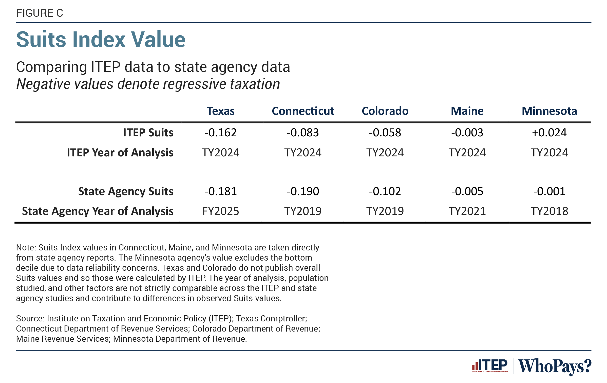
The Suits Index values derived from the studies produced by various state agencies are not far off from the values calculated in this study. The findings from Texas, Connecticut, and Colorado are in agreement with the findings of this study indicating that each of those states’ tax codes is meaningfully regressive. In Maine and Minnesota, which have robust income taxes and income-based offsets to their property taxes, ITEP and the relevant state agencies agree that the overall systems come closer to proportionality overall, with both progressivity and regressivity present at various points along the income scale.
The most notable difference between the state agency studies and this study is that the states’ tax incidence studies find somewhat more regressivity. One factor likely contributing to this finding is the exclusion of seniors from this study. As discussed earlier, seniors may face higher consumption and property tax rates if their ratios of spending to income, and home value to income, are higher than for non-seniors. Higher tax rates under these regressive tax sources would tend to increase the overall measure of regressivity present in the tax code.
The year of analysis is also an important consideration in many of these states. The Minnesota Department of Revenue study, for instance, was published in March 2021, using 2018 base year data, and therefore does not include the effects of progressive tax legislation enacted in 2023. Using the supplementary data contained in Appendix D of this study, we find that the Minnesota tax code as it existed in 2018 had a Suits Index value of +0.004—an amount that is nearly indistinguishable from the -0.001 value found in the Minnesota report.
A similar issue is present in the Colorado and Connecticut studies, both of which analyze 2019 tax law. Colorado and Connecticut enacted meaningful tax cuts for low-income families in recent years that are included in this study but were outside the scope of the state agency studies. Colorado also enacted a variety of progressive personal income tax reforms in 2021 affecting high-income families’ capital gains, pass-through business income, and itemized deductions. It is likely that future editions of these two studies will show somewhat less tax regressivity due to these reforms and that their results will move toward Suits values even closer in line with those found in this study.
A central reason for the broad similarities in results seen across these studies is the consensus among them that consumption and property taxes tilt in a regressive direction. In all these studies, sales and excise taxes are found to be regressive—the most regressive major sources of revenue in most of them. The Texas Comptroller, for instance, finds that the bottom quintile of Texas residents pay more than 4 times as much, measured as a share of household income, in sales and use taxes than the top quintile. While personal income taxes can mitigate tax regressivity in states choosing to levy them, in practice these taxes are not robust enough to produce a genuinely progressive overall outcome. This is why all five of the most comprehensive tax incidence studies produced by state agencies find their states’ tax codes to be regressive overall.
The key takeaway of these comparisons is that, among the organizations that have studied state and local tax incidence most closely, there is wide agreement on the distributional shape of those tax codes. The typical state and local tax code is undoubtedly regressive, though this outcome can be avoided with robust income taxation and the provision of income-based property tax offsets, as is the case in Maine and Minnesota.
Section 3: Alternative Presentation With Exported Taxes
The results reported in this study show the distribution of state and local taxes paid by residents to the states in which they live. This analysis allows lawmakers to understand how the tax laws they help write are impacting their constituents and allows residents to see how their state’s taxes are affecting them relative to others in their state. This kind of analysis is best suited to answer the most pressing questions that state and local lawmakers have about tax distribution and to better inform voters about the policies their state has control over.
From a national perspective, it is also worth examining the distributional impact of cumulative taxes paid by residents to all states—including the taxes that are “exported” from states other than their own. Figure D offers an alternative presentation of the data that includes this information. It shows that the regressive impact of state and local taxation remains little changed when exported taxes are included. Adding exported taxes increases the effective rate on low-income families by 2.2 percentage points while it raises the effective rate for the top 1 percent by 2.6 percentage points. Overall effective tax rates rise to 13.6 percent of income for low-income families and to 9.7 percent of income for high-income families—a slightly less regressive result than without considering exported taxes.
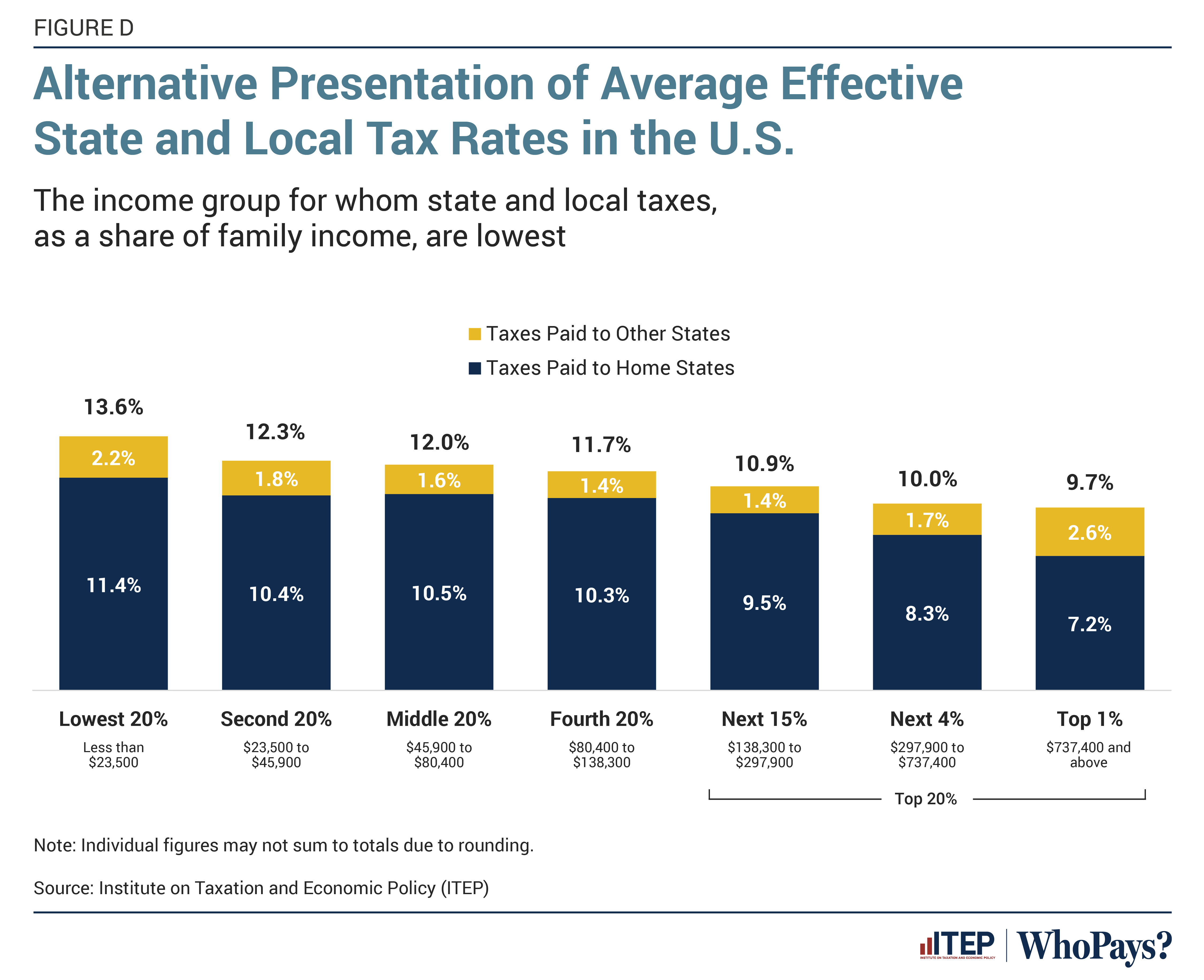
This muted distributional impact is driven by the wide diversity of tax types being exported, and the wide variety of mechanisms through which that exporting occurs. High-income taxpayers, for example, pay taxes to other states when they own stock in a corporation that pays another state’s corporate income tax, or when they own a vacation home outside of their home state that is subject to property taxes. Low- and middle-income taxpayers are impacted more noticeably by other states’ sales taxes and diesel fuel taxes, which can raise the cost of goods being shipped into their state from other parts of the country. And a broad swath of people pay tax directly on their gasoline, restaurant meals, and other purchases when they travel outside of their home states to visit family or take a vacation.
Section 4: The ITEP Inequality Index
The ITEP Tax Inequality Index measures the effects of each state’s tax system on income inequality. It aims to answer the following question: Are incomes more, or less, equal after state and local taxes are collected? For each state, the Index compares incomes by income group before and after taxes.
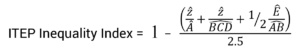
Specifically, our measure is one minus a weighted average of three measures of relative tax preference:
1. The wealthy to the poor, by comparing the top 1 percent to the bottom 20 percent
2. The wealthy to the middle class, by comparing the top 1 percent to the middle 60 percent
3. High earners to low- and moderate-income families broadly, by comparing the top 20 percent to the bottom 40 percent, half weighted
Therefore for:
- The five quintiles of income = {A, B, C, D, E}
- The top percentile of income = z
- x̂ = after-tax income as a share of pre-tax income
States with regressive tax structures have negative ITEP Index values, meaning that incomes are less equal in those states after state and local taxes than before. States with progressive tax structures have positive Index values; incomes are more equal after state and local taxes than before.
The ITEP Index is not the only measure of state and local tax regressivity, but it does have advantages over the other indices that lead us to use it as the benchmark across states for this study.
The Suits Index is the most used overall measure of tax regressivity at the state level (Suits, 1977). As with the ITEP Index, Suits evaluates taxes relative to income across the income distribution. But it does so by comparing each income group’s share of income to its share of taxes paid and calculating the cumulative difference between those two measures.
For instance, if the bottom 20 percent of tax units collect 3 percent of income but pay 6 percent of a given state’s taxes, Suits would correctly label the effect of those taxes as regressive for this segment of the income distribution. Requiring such outsized payments, relative to income, by families of very modest means risks worsening the economic hardship that they are likely already confronting and should be front of mind for lawmakers considering the disparate effects of the tax law across the economic spectrum. But in the Suits calculation, this group’s tax payment has only a minor effect on the overall result because their contribution to the tax’s final Suits value is constrained by the fact that 97 percent of income received and 94 percent of taxes paid were associated with other groups. In other words, the mathematical construction of Suits fails to give adequate weight to the outsized human toll that comparatively high tax rates can have on families in vulnerable economic situations.
Less frequently cited in state tax distributional work, but also of note, is the Kakwani Index (Kakwani, 1977). Developed around the same time as Suits, Kakwani is less prone to minimizing the importance of tax policy for economically vulnerable families because it measures tax distribution in proportion to the share of households.
Taking the above example, in the Kakwani Index tax rates on the bottom 20 percent of households have more sway over the final Index value simply because this group comprises 20 percent of households—the fact that they only receive 3 percent of income does not work against them in the same way that it does under Suits.
With Kakwani, however, the main disadvantage arguably lies at the other extreme end of the income scale. Taxation of the top 1 percent of earners is a key practical consideration for state tax policymakers because this group receives a large share of income, but the taxation of that income has comparatively little effect on the Kakwani Index since this group represents such a small share of overall households.
The ITEP Index strikes a balance between these two approaches by providing somewhat more weighting at the very bottom of the income scale than does the Suits Index (where the human toll of regressive taxation is highest), and somewhat more weight to the top of the income scale than does the Kakwani Index (where tax rates matter most to revenue capacity).
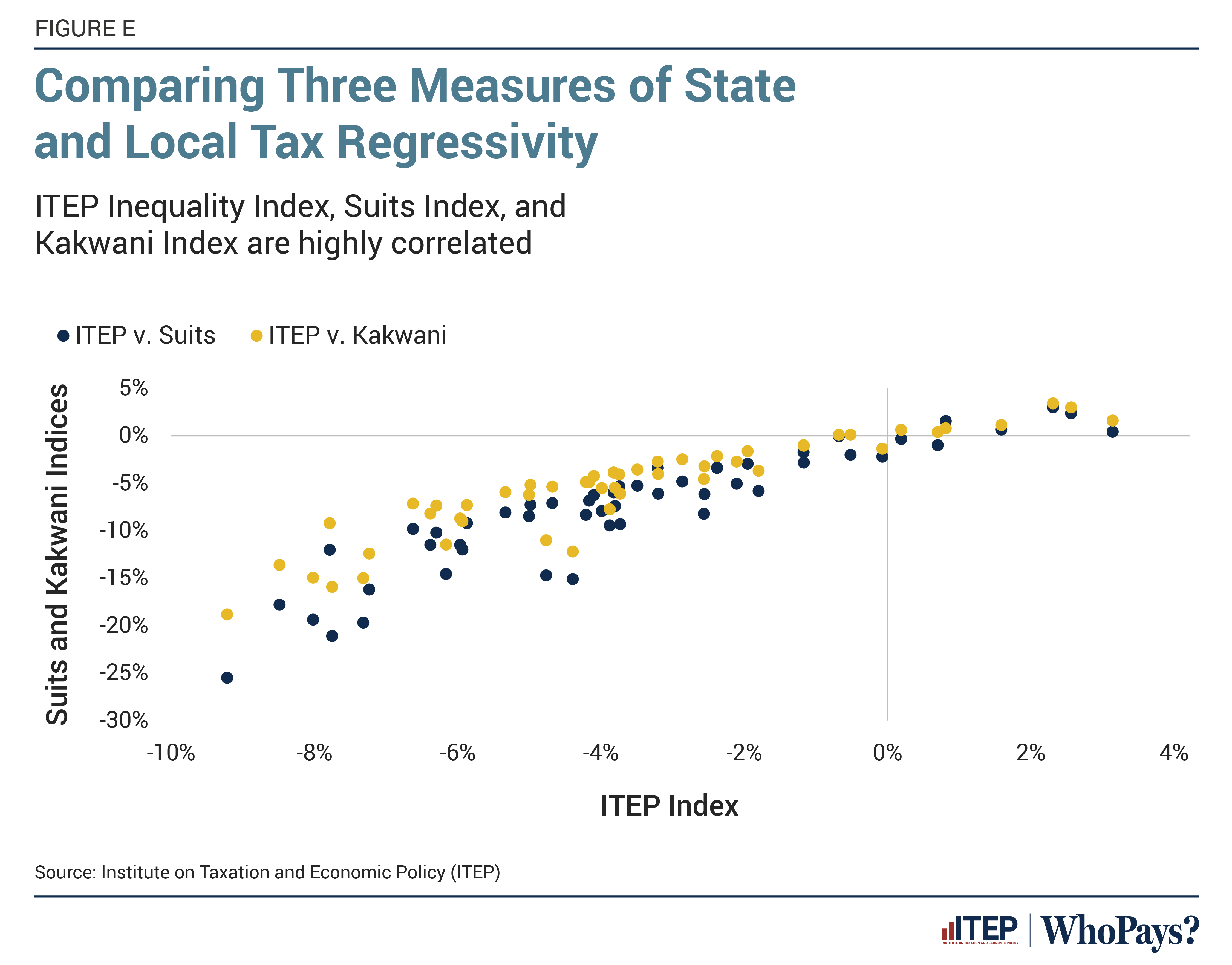
Ultimately, each of these methods are attempting to measure the same concept, as evidenced by the high degree of correlation between these measures exhibited in Figure E. In this figure, each dot represents a state and, regardless of the measure chosen, the same pattern holds. States that are more regressive under the ITEP Index, and therefore appear on the left side of the chart, are also more regressive under the other two measures. All three measures point toward meaningful levels of regressivity in the large majority of state and local tax systems.
Appendix G References
Bartik, Timothy (2009). “What Works in State Economic Development?.” In Growing the State Economy: Evidence-Based Policy Options, 1st edition, edited by Stephanie Eddy and Karen Bogenschneider. Madison, WI: University of Wisconsin, 15-29.
Besley, Timothy J., and Harvey S. Rosen (1998). “Sales Taxes and Prices: An Empirical Analysis.” National Tax Journal 52 (2), 157-178.
Black, David E. (1974). “The Incidence of Differential Property Taxes on Urban Housing: Some Further Evidence.” National Tax Journal 27 (2), 367-369.
Brewer, Ben K., Karen Smith Conway , and Jonathan C. Rork (2017). “Protecting the Vulnerable or Ripe for Reform? State Income Tax Breaks for the Elderly: Ten and Now,” Public Finance Review 45(4), 564–594.
Brock, Betsy, Kelvin Choi, Raymond G. Boyle, Molly Moilanen, and Barbara A. Schillo (2016). “Tobacco Product Prices Before and After a Statewide Tobacco Tax Increase.” Tobacco Control 25, 166-173.
Buis, Maarten (2017). “FMLOGIT: State module fitting a fractional multinomial logit model by quasi maximum likelihood.” Boston College Department of Economics.
Burman, Leonard B., Katherine Lim, and Jeffrey Rohaly (2008). “Back from the Grave: Revenue and Distributional Effects of Reforming the Federal Estate Tax.” Tax Policy Center.
Chainbridge Software (2013). “Chainbridge’s Approach to Modeling State Sales Tax Policy Changes.” The Federation of Tax Administrators Revenue Estimation and Tax Research Conference.
Charles, Kerwin Kofi, Sheldon Danziger, Geng Li, and Robert F. Schoeni (2007). “Studying Consumption with the Panel Survey of Income Dynamics: Comparisons with the Consumer Expenditure Survey and an Application to the Intergovernmental Transmission of Well-being.” Federal Reserve Board.
Chouinard, Hayley, and Jeffrey M. Perloff (2004). “Incidence of Federal and State Gasoline Taxes,” Economics Letters 83, 55-60.
Cline, Robert J., Andrew D. Phillips, Joo Mi Kim, and Thomas S. Neubig (2010). “The Economic Incidence of Additional State Business Taxes.” Tax Analysts Special Report, 105-126.
Colorado Department of Revenue (2022). “2022 Tax Profile & Expenditure Report.”
Connecticut Department of Revenue Services (2022). “Connecticut Tax Incidence Study – Tax Year 2019.”
De Agostini, Paola, Bart Capéau, André Decoster, Francesco Figari, Jack Kneeshaw, Chrysa Leventi, Kostas Manios, Alari Paulus, Holly Sutherland, and Toon Vanheukelom (2017). “EUROMOD Extension to Indirect Taxation: Final Report.” Euromod Technical Note Series.
Eltinge, J. L., Westat Yansaneh, and G. D. Paulin (1994). “Assessment of Reported Differences Between Expenditures and Low Incomes in the U.S. Consumer Expenditure Survey.” Proceedings of the Survey Research Methods Section, American Statistical Association.
Hanson, Andrew and Ryan Sullivan (2009). “The Incidence of Tobacco Taxation: Evidence from Geographic Micro-Level Data.” National Tax Journal 62 (4), 677-698.
Hyman, David N. and Ernest C. Pasour, Jr. (1973). “Property Tax Differentials and Residential Rents in North Carolina.” National Tax Journal 26 (2), 303-307.
Johns, Andrew and Joel Slemrod (2010). “The Distribution of Income Tax Noncompliance.” National Tax Journal 63 (3), 397-418.
Kakwani, Nanak C. (1976). “Measurement of Tax Progressivity: An International Comparison.” The Economic Journal 87 (345), 71-80.
Kenkel, Donald S. (2005). “Are Alcohol Tax Hikes Fully Passed Through to Prices? Evidence from Alaska.” American Economic Review 95 (2), 273-277.
Krause, Melanie R., Barry W. Johnson, Peter J. Rose, and Mary-Helen Risler. “Federal Tax Compliance Research: Tax Gap Estimates for Tax Years 2014-2016.” Internal Revenue Service Publication 1415 (Rev. 08-2022).
Li, Geng, Robert F. Schoeni, Sheldon Danziger, and Kerwin Kofi Charles (2010). “New expenditure data in the PSID: comparisons with the CE.” Monthly Labor Review, Bureau of Labor Statistics, 20-30.
Maine Revenue Services (2023). “Maine State Tax Expenditure Report 2024-2025.” Reports Prepared for the Joint Standing Committee on Taxation.
Minnesota Department of Revenue (2021). “2021 Minnesota Tax Incidence Study: An Analysis of Minnesota’s Household and Business Taxes Using November 2020 Forecast.” Minnesota Department of Revenue Tax Research Division.
Orr, Larry L. (1970). “The Incidence of Differential Property Taxes: A Response.” National Tax Journal 23 (1), 99-101.
Parker, Justin (2020). “Natural Gas Markets Remain Regionalized Compared with Oil Markets.” U.S. Energy Information Administration, Today in Energy.
Rogers, John and Maureen B. Gray (1994). “CE data: quintiles of income versus quintiles of outlays.” Monthly Labor Review, 32-37.
Suárez Serrato, Juan Carlos, and Owen M. Zidar (2023). “Who Benefits from State Corporate Tax Cuts? A Local Labor Market Approach with Heterogeneous Firms: Further Results.” National Bureau of Economic Research, Inc. NBER Working Paper 31206.
Suits, Daniel B. (1977). “Measurement of Tax Progressivity.” The American Economic Review 67 (4), 747-752.
Texas Comptroller of Public Accounts (2023). “Tax Exemptions & Tax Incidence.”
Wasylenko, Michael and Therese McGuire (1985). “Jobs and Taxes: The Effect of Business Climate on States’ Employment Growth Rates.” National Tax Journal 38 (4), 497-511.
Weinstein, Bernard L (1984). “Who Pays the Severance Tax?.” Policy Studies Journal 12 (3), 537-545.